
Shrimp grading using a robotic arm and computer vision
A station by station map for Indian processors: the count per pound grade verification pipeline, the vision system specification with parameters and fallbacks, and a 16 point vendor checklist for a shrimp line.
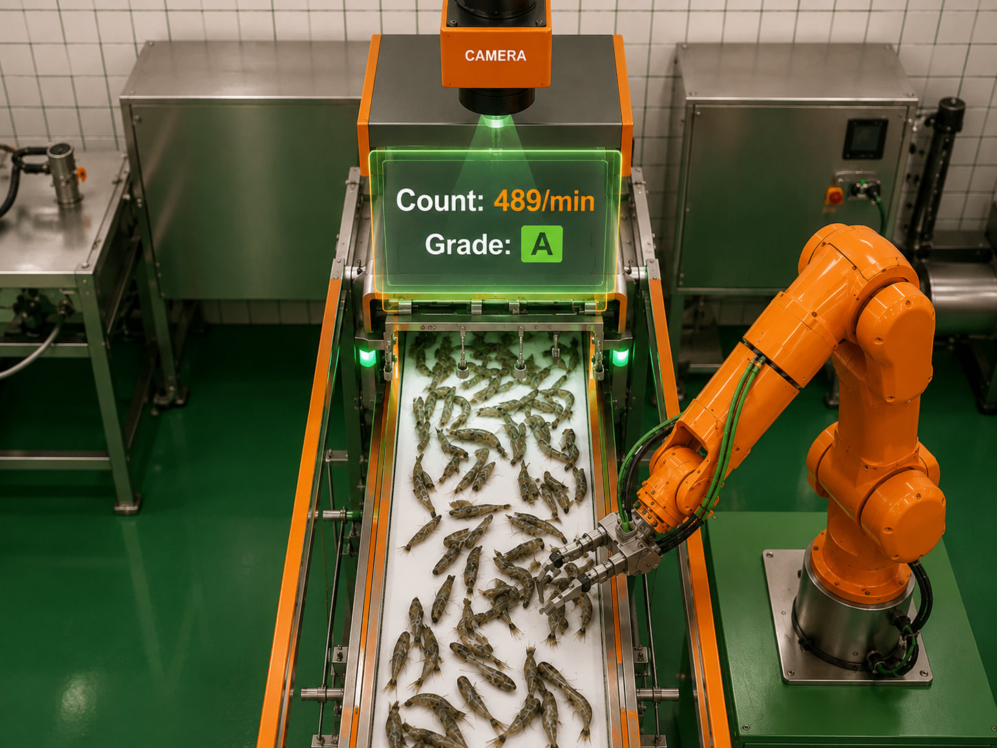
A 40 to 60 MT/day Indian shrimp plant runs several hundred workers across deheading, peeling, deveining, grading and packing, QC by sampling and eye. Labour is ₹10,000 to 15,000 per worker per month. At that price, automation that only replaces headcount rarely pays back, and loses money if it costs yield. Raw material is 70 to 80% of cost; margins are low single digits.
The target is not headcount but measurement: recovering lost yield, capturing unrealised price, catching losses (rejections, claims, failed audits) before shipping. This page maps the line, then details the highest payback pipeline: grade verification. The line detail here comes from our pilot work with Danica Aqua Marine, Visakhapatnam.
Where labour replacement automation fails
Automatic deheading lines quote up to 70% lower labour cost and 2 to 3 times manual throughput. A peeling line cuts 100 manual workers to about 40, fewer on a PUD line. Removing 60 workers at ₹12,000/month saves about ₹86 lakh a year.
But automatic peeling yields 3 to 5% below hand peeling, mostly at the tail tip. With raw material at 70 to 80% of cost and margins of 2 to 4%, that loss can exceed the labour saved. So plants stay manual, and the useful vision work measures the process, not replaces it.
What is already sold, and its limit
| Category | Examples | Does | Does not |
|---|---|---|---|
| Optical sorters | TOMRA, Bühler, Key Technology | Eject peel, shell, legs, eyes, tails, by catch from a bulk flow. ₹1.5 cr and up. | Verify count per pound, assess incoming lots, attribute yield, per batch audit |
| Peeling / deveining | Laitram, Gregor Jonsson | Peel 10 to 90 count, all product forms, up to 10x hand speed | Load themselves (manual), measure anything |
| Grading / weighing | Marel | Grade by physical dimension, weigh, batch | Measure count per pound (dimension is a proxy, not the count) |
| Regional lines | Yuanyu, Foshan Soontrue, Powertech | Deheading and PD lines at low cost | Measure the process |
Optical sorters eject product from a flow. None measure the process producing it. Retrofit vision does, at ₹5 to 15 lakh, on a line already running and paid for.
The line at a glance
| Station | Status | Where vision fits | Cost |
|---|---|---|---|
| Receiving | Perception | Per lot size distribution, count per pound estimate and melanosis incidence from a sampling tray, in a 60 second report at the point of purchase | ₹4 to 8 L |
| Deheading | Mechanisable | Cut position monitoring: yield loss per table, shift and operator (management data, not machine control) | ₹5 to 9 L |
| Peeling | Machine solved | Loading the machine is manual; robotic singulation of wet, clumped shrimp is an open research problem, not a product | ₹35 to 45 L |
| Grading | Perception | Count per pound verification. The pipeline below. | ₹12 to 15 L |
| Melanosis | Perception | Per pack black spot incidence and severity, added as a class on the grading install | ₹6 to 10 L |
| Weigh / pack | Weighing solved | Timestamped, batch indexed audit record for BRC and BAP | On grading install |
| Metal detection | Solved | Surface plastic and organic debris that X ray misses (complements, does not replace, metal detection) | ₹4 to 7 L |
| Palletising | Mechanisable | Six axis cobot with vacuum tool. Labour based payback, so weak in India | ₹35 to 45 L |
Washing, soaking, IQF freezing, glazing and cold store use standard equipment, no vision needed. The rest of this page is the grading pipeline, the largest and most direct return.
Grading: the highest value case
Price is set by count per pound: bands like 16/20, 21/25, 26/30, a lower number meaning larger shrimp and higher price per kilogram. Mechanical roller and weight graders sort by physical dimension, a proxy for count. The two diverge with moisture, soaking uptake, product form (head on, headless, tail on) and size spread within a band. A pack one band low gives away margin; one band high draws a buyer claim.
At ₹135 to 140 crore annual revenue, a 0.5% grade realisation gap is about ₹68 lakh, roughly a quarter of the year’s profit at a 2% margin. A 0.2% gap is ₹27 lakh. A 2% gap, which is not unusual, erases the year’s profit.
The pipeline
- Capture. Overhead global shutter camera (2 to 5 MP, 30 to 60 fps) over the grading discharge or sampling tray, fixed working distance, controlled LED, a colour and scale reference card in frame for per frame calibration.
- Instance segmentation. Isolate every shrimp, including touching ones, into per object masks. Model: Mask R-CNN or a YOLO-seg / RTMDet-Ins class network trained on plant imagery. Clumped clusters are flagged and excluded from the count, not guessed.
- Morphometry. Per mask: medial axis length with curvature correction (a spline fitted to the skeleton straightens the curl), projected area, and mid body width.
- Weight and count. Convert size to individual weight with a calibrated length weight model W = a·Lⁿ or a small learned regressor. Count per pound is 453.6 divided by mean individual weight in grams. The grade band follows, with an explicit interval from quantile regression or an ensemble.
- Per pack verdict. Aggregate over a pack or batch window: measured count distribution against the declared band, percent in band, and the direction of any miss.
Deriving weight: 2D or 3D
Sizing accuracy is won or lost here, and the sensor sets the ceiling. Grade is count per pound (weight), not what a mechanical grader measures. Three options, descending in accuracy and cost:
| Method | How weight is derived | Weight target | Use when |
|---|---|---|---|
| 3D: laser profile or RGB D | Recover volume, then a volume to weight regression | ± 3 to 5% | Multiple product forms, or soaking in use |
| 2D morphometry | Instance segmentation, then length, area and a curvature corrected axis to a per grade weight regression | ± 5 to 8% | A stable single product form |
| 2D length only | Length against a lookup table, a dimensional proxy | Cross check only | Verification against another method, never a primary claim |
Sizing is commonly specified as 95% correct grade band assignment. That figure means nothing without its method: ask how it is measured, and against what reference.
Calibration. Coefficients are fit against physically counted and weighed reference trays, never the grader’s own output, which would propagate the error being measured. Recalibration is scheduled, as size distribution and shell condition drift across the culture cycle.
Data required. 20,000 to 30,000 annotated instances across at least five grade bands and both major product forms, plus weighed reference trays for ground truth.
Targets, benchmarked in the proof of concept. Count per pound mean absolute error within about one count for most packs; per pack verdict in seconds; throughput matched to the grading line in shrimp per hour. Numbers to benchmark against, not claimed results.
From real time verdicts to the end of run report
The system produces two things. In the run it emits a verdict per pack in real time: pointers that raise an alert, drive an air jet, or light a screen indication. These are operational, not the deliverable.
The deliverable is a report, finalised at a logical endpoint rather than streamed: a batch or grade change, line stop, or shift end. At that trigger the system closes the window, aggregates its verdicts, reconciles counts against the window’s weighed reference samples, and generates one report per line and batch, readable by an owner, not only a QC head. It carries:
- Grade realisation. Declared band, measured count distribution, percent in band, percent graded low (margin lost), percent graded high (claim risk).
- Value in rupees. Low and high grading converted to money against the day’s price sheet. The first line an owner reads.
- Count per pound histogram per band, showing spread and outliers.
- Attribution. Which line or grading station is drifting, so it can be reset the same day.
- Shift trend. Morning against evening, to catch drift from ice melt, fatigue or throughput changes.
- Defect incidence. Melanosis and foreign material percentages, if those classes are enabled.
- Batch and lot identity. Which run this is, its declared grade and product form, start and stop times.
- Throughput and coverage. Pieces assessed, and the percent abstained on for clumping, so the report states its own sampling.
- Exceptions. Packs the system could not assess, listed rather than silently dropped.
- Audit record. Every verdict timestamped and batch indexed, exportable for BRC and BAP.
It is generated automatically at the trigger, sent to owner and QC head as a one page summary with the full record attached, and kept as the batch audit trail. Nothing depends on an operator remembering to compile it.
Melanosis: grading black spot, and where we start
Melanosis, the black spot that forms on head and shell within hours of harvest, is enzymatic browning driven by polyphenol oxidase. It is scored 0 to 10 (Otwell and Marshall): 4 is a measurable defect, 8 approaches reject grade. A leading cause of consignment downgrade, with one review putting darkened product at around 10% of export weight. Sampling QC catches the batch average, not the per pack incidence that triggers a buyer claim.
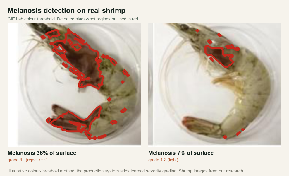
The method. Naive RGB thresholding fails: black spot overlaps in RGB with ice glare, wet shell sheen, shadow and natural cephalothorax pigment. What works: illumination normalised CIE Lab colour, texture descriptors, and learned segmentation that grades severity rather than yes or no. The hard part is class imbalance: affected product is often under 2% of throughput, so per class sensitivity, not overall accuracy, is the metric.
Three method tiers, in descending order of what they deliver and demand:
| Approach | Output | Limitation |
|---|---|---|
| Learned segmentation (Mask R-CNN or YOLO-seg) | Per pixel spot masks, a severity score per piece on the 0 to 10 scale | Needs a substantial labelled dataset |
| Colour space thresholding (CIE Lab) | Percentage of affected surface area, with illumination normalisation and a texture descriptor to separate spot from shadow | Weak on early stage spot and on natural dark pigmentation |
| Binary flagging | Presence or absence at pack level, an audit flag | No severity, no localisation |
The data problem. Affected product is often under 2% of throughput, so overall accuracy is meaningless and both training and validation are statistically awkward. Insist on per class sensitivity and precision against expert labelled ground truth, and deliberately source rejected and downgraded lots: a model trained only on good product cannot detect bad product.
Where we start: the data. The scarce input is labelled shrimp imagery under real conditions, which we have been building: a growing corpus from the local Visakhapatnam cluster, hatcheries and farms, spanning size grades, freshness states and melanosis severities. It lets us stand up a melanosis or grading model quickly and validate it against a plant’s own QC, not from zero. The detectors are at proof of concept stage, benchmarked pack by pack before anything is trusted.
Beyond melanosis: the full defect sheet
Melanosis is one visual defect among many. Buyers grade against a defect sheet; a shrimp is rejected for any deviation from spec: attached shell, discolouration, black gill and black head, dropping or loose head, vein not removed, dehydration and freeze burn, clumping, soft shell, deep cuts, broken pieces, foreign matter, and count or size out of grade. Each defect carries a tolerance limit and a class (critical, major or minor); the defect percentage is defective units over sample size, judged against an agreed AQL, critical defects targeted at zero.
A vision layer screens the visual defects on every pack, not one sampled carton, and logs each to the defect sheet automatically. It does not cover smell, decomposition below the surface, or chemical and microbial residues, which stay with the lab and human grader.
For structural defects (broken pieces, deep cuts, loose heads, shell fragments on peeled product, incomplete deveining), three approaches apply, and a new site usually starts with the last:
| Approach | Best for | Note |
|---|---|---|
| Anatomical modelling | The long tail of defect types | Instance segmentation with a shape descriptor compared against a learned model per product form |
| Contour analysis | Gross breakage | Perimeter, aspect ratio, convexity deficit, segment count; transparent and cheap |
| Anomaly detection | New plants with no labelled defect data | Trained only on good product; flags deviation without classifying it |
Anomaly detection suits a new site. It needs no defect examples. It flags that something is wrong rather than what, acceptable in a manual assist deployment and running months earlier. Classes differ by line: HOSO work on head and gill discolouration, loose heads and broken antennae; peeled and deveined lines on vein residue, meat tears from the peeler, and tail on completeness.
| Defect | Surface vision? | Note |
|---|---|---|
| Count / size out of grade | Yes | The core case: per object sizing and count per pound |
| Melanosis (black spot) | Yes | Severity on the 0 to 10 scale, per pack |
| Black gill / black head | Yes | Localised discolouration at gill and head |
| Discolouration | Yes | Colour deviation from the spec |
| Attached shell, shell in PUD | Yes | Shell fragments on peeled product |
| Dropping / loose head | Yes | Head separation on head on product |
| Deep cut / broken / damaged | Yes | Shape and edge break detection |
| Dehydration / freeze burn | Yes | Surface whitening and texture |
| Clumping (IQF) | Yes | Pieces frozen together |
| Vein not removed | Partly | Only where the vein shows on the surface |
| Soft shell | Partly | An appearance cue, not a definitive test |
| Foreign matter | Partly | Surface only; sub surface needs X ray |
| Bad smell / odour | No | Not a visual property |
| Decomposition (early) | No | Only advanced stages reach the surface |
| Antibiotic / microbial residue | No | Needs a lab assay, not imaging |
One camera platform can carry many of these as separate trained classes on one install, so grading, melanosis and the surface defect set run together, not as separate machines. The discipline: claim only the visual set and the count; leave smell, decomposition and residues to the methods built for them.
How to specify the system
Most vision projects on a food line fail for one of three reasons: motion blur at line speed, specular glare from wet product, or a model that validated in commissioning week and drifted by month three. None are vendor specific; all are visible in advance, and are specification failures, not bad luck. Each section below gives the parameter that matters, an indicative target, and the fallback when site or budget rules out the ideal.
Every fallback costs a capability. Stating it puts the compromise in the scope document, not the acceptance meeting.
Start with the line rate
Every other number follows from this. A line at 500 pieces per minute presents 8.3 per second. If the inspection zone is 400 mm and the belt runs at 0.5 m/s, each piece sits in the field of view for roughly 800 ms: ample in principle, none at all if the camera cannot freeze it. Three measurements precede any specification:
- Belt speed (m/s), from an encoder or timed marker. Sets the exposure and frame rate requirement.
- Pieces per minute, counted over 60 seconds three times. Sets the processing throughput.
- Belt area coverage (%), photographed and estimated. Determines whether clumping is the gating problem.
Camera and optics
The sensor and lens follow the line rate measured above.
| Parameter | Target | Fallback | What the fallback costs |
|---|---|---|---|
| Sensor | Industrial global shutter CMOS | Global shutter at a lower frame rate, belt slowed locally | Throughput, not accuracy |
| Resolution | 2 to 5 MP, sized so the smallest defect spans at least 8 to 10 pixels | Wider field of view split across two cameras | Money, not capability |
| Frame rate | At least 60 fps at full resolution | 30 to 40 fps on a slowed inspection zone | A line modification |
| Lens | C mount, focus and aperture mechanically locked | None: unlocked optics drift within weeks under vibration | Focus and scale calibration |
| Enclosure | IP67 minimum, IP69K preferred | IP65 with a secondary shroud | Washdown tolerance and service life |
Interface. GigE Vision or USB3 Vision; either is standard, the choice following the cable run and controller.
The test that decides shutter type. Capture frames at production speed and measure motion blur. If a shrimp smears more than about one pixel along travel, a rolling shutter will not work and no software recovers it. Rolling shutter works only with strobed illumination short enough to act as the effective exposure, and even then do not claim detection of melanosis spots under 2 mm.
Illumination
Illumination is the item most often underspecified, and it sets the ceiling on everything downstream. Wet chitin is close to a mirror: untreated, specular highlights destroy colour fidelity and edge detection, so the system reads glare as a defect and a shadow as a spot.
| Aspect | Target | Fallback | What the fallback costs |
|---|---|---|---|
| Geometry | Enclosed tunnel or dome, white diffuse inner surface | Open diffuse bar with an ambient light shroud | Colour based classes degrade |
| Source | High intensity LED bars, strobed in sync with the shutter | Continuous diffuse LED | Effective exposure lengthens, blur risk returns |
| Glare control | Cross polarisation: a linear filter on both source and lens | Diffusion only, no polarisation | 1 to 2 stops of contrast on wet shell; melanosis severity unreliable |
| Ambient isolation | Sealed from hall lighting | Shroud only | Model drifts as hall light changes across the shift |
Required at every tier: a fixed white and grey calibration reference in the field of view. Near zero cost, and the only practical way to detect and correct illumination drift as lamps age and doors open.
Decision trigger. If specular highlights cover more than roughly 15% of shrimp surface area in your frames, cross polarisation is not optional.
Clumping and singulation
Clumping is the hardest perception problem on the line, and the one most often passed over in a quote. Solve it mechanically first: a vibratory spreader or belt speed differential that separates product before the inspection zone turns a hard problem into an easy one, as established sorting lines rely on. Where that is impossible, two software positions are defensible, both stated for what they are:
- Confidence gating. The system abstains on heavily overlapped clusters and passes them through rather than guessing. A cluster reported as unassessed is more useful than one guessed at.
- Top layer assessment. Inspect the visible layer and report coverage percentage with the result. This is a sampled measurement and must be stated as one.
Decision trigger. Above roughly 30% belt area coverage, no software approach is reliable. Either fix the presentation or reduce the claim.
Processing and latency
Inference runs on site, always.
- Inference latency: at most 15 ms per frame, which sets the reject timing budget.
- Hardware: an industrial edge module (for example an NVIDIA Jetson Orin class device) or a rugged x86 with an entry GPU.
- Runtime: ONNX Runtime or TensorRT.
- Cloud processing: not acceptable for in line decisions; latency and plant connectivity both rule it out.
For detection and report applications (receiving bay lot assessment, audit logging, grade verification without actuation) CPU only inference on commodity hardware is viable at reduced frame rates. That drops the GPU from the bill of materials and puts a camera only system in a far lower capital bracket. Not every application needs an Orin.
Rejection
The rejection mechanism is chosen against the line rate, not the other way round.
| Mechanism | Sustained rate | Actuation time | Requirement |
|---|---|---|---|
| Pneumatic air jet | 500+ pieces/min | At most 5 ms valve response | Clean, dry, oil free air at 5 to 6 bar through food grade filtration |
| Mechanical paddle or diverter | 200 to 400/min | 20 to 50 ms | No air |
| Manual assist (projected light, laser marker or screen) | Any rate, operator limited | n/a | No air |
Robotic picking is not a rejection mechanism at line speed: a high speed delta cell sustains roughly 150 to 200 picks per minute against a line presenting 500. Robots belong where the task is placement (tray loading, orientation, pack presentation), not rejection; the two should not be conflated in a specification.
Line integration
Three integration modes, matched to how far a plant will open its line to a supplier:
- Full PLC integration. Profinet or Modbus TCP, a deterministic timing loop and encoder based belt tracking, for plants willing to open the PLC to a vendor.
- Digital I/O trigger. The vision controller signals an existing reject controller. This fits most retrofits.
- Report only. Display, alarm and a logged record, no actuation. The correct mode for a first installation.
Encoder tracking lets the system fire on the right piece rather than at the right moment; without it, reject accuracy degrades as belt speed varies. Most processors will not grant PLC access to a first time supplier, so plan for report only in project one and integration in project two.
Deploying it
One project that automates a whole plant is how automation projects fail. The order that works, none of the early steps needing a robot:
| Phase | Scope | Cost |
|---|---|---|
| 0 | Proof of concept: one station, three weeks, accuracy report vs your QC | ₹2 to 2.5 L |
| 1 | Permanent grading verification station | ₹12 to 15 L |
| 1b | Additional stations on the same platform | ₹8 L each |
| 2 | Automated rejection: air blast or pusher on the belt | ₹6 to 10 L |
| 3 | Vision guided robotic handling or palletising cell | ₹35 to 45 L |
Nothing actuates on a detection until it has run in report only mode for a full season. A model at 88% sensitivity is a useful report; the same model driving a rejector discards good product 12% of the time.
What the plant provides: station access during production, 230V within a few metres, a clamp fixed camera mount (no drilling, IP65), one QC person for benchmarking, permission to record imagery including bad lots, and weighed reference samples. About two days of access over the three weeks, ideally off peak (Andhra cycles peak February to May and August to November).
Drift, revalidation and cross plant generalisation
A model that passes at commissioning can fail quietly later. Known drift sources on a shrimp line: seasonal morphological variation across the culture cycle, lamp ageing and changing ambient light, belt wear altering the background, pond source and feed variation between suppliers, and changes in soaking or treatment practice.
The specification against drift is concrete: an in frame calibration reference, continuous illumination normalisation, an automated drift alarm, and scheduled revalidation each production season against fresh expert labels. Revalidation should be a named line item with a price, not an unbounded obligation in a support contract, for the supplier’s sustainability as much as the buyer’s clarity.
A model trained at one processor routinely underperforms at another: pond source, feed, size distribution, belt speed, lighting geometry and product form all differ. Assume per site fine tuning on two to three shifts of local data over a shared base model, and check it is priced in. A vendor deploying an unchanged base model is describing a demonstration, not an installation.
The vendor checklist
Sixteen questions for a vendor meeting. A vendor who answers all sixteen without hedging is worth talking to. One who quotes a single headline accuracy number and nothing else is not.
- Shutter and frame rate. Global or rolling shutter, and what frame rate at our measured line speed?
- Motion blur. What is the measured motion blur, in pixels, on our product?
- Glare. How is specular glare from wet shell handled: polarisation, diffusion, or neither?
- Calibration reference. Is there a calibration reference in the field of view?
- Sizing method. Is sizing 3D or 2D, and how is weight derived?
- Sizing ground truth. How is sizing ground truth established, and is it independent of our existing grader?
- Melanosis output. Is melanosis reported as severity or presence, and against whose grading scale?
- Per class metrics. Per class sensitivity and precision, not overall accuracy?
- Defect data. How is the defect training set sourced, given defect rates below 2%?
- Clumping. What happens when product is clumped: does the system abstain or guess?
- Latency. Inference latency per frame, on what hardware, on site?
- Rejection. Reject mechanism, valve actuation time, air specification?
- Belt tracking. Is belt tracking encoder based?
- Revalidation. What is the revalidation schedule, and its cost?
- Fine tuning. Is the model fine tuned on our data, or deployed as is?
- Enclosure. Enclosure IP rating, and washdown chemical compatibility?
Frequently asked questions
Every project starts with a proof of concept, usually two weeks to a month, its timing set by how fast you can supply the data and how clean it is. Once it holds up, we build it into a full system around the needs it surfaced.
Working with us
We run paid, fixed scope proofs of concept at one station, three weeks, with defined deliverables and an accuracy report benchmarked against your QC team. The fee is adjustable in full against a later deployment.
Before that, at no cost: send ten minutes of footage from your grading table or receiving bay. We return an analysis of what is detectable on your line, what is not, and what it would take.
Send footage for a free line reviewThe platform does real time perception on commodity hardware, edge or CPU inference, no customer GPU, from standard IP cameras over RTSP and ONVIF. Ethan AI built it for behavioural state detection in clinical settings, and part of the proceeds from this consulting work funds that research. Clinical figures do not transfer to shrimp; the architecture and the practice of validating against expert labels do.